Random Forest 随机森林
Theroy 原理
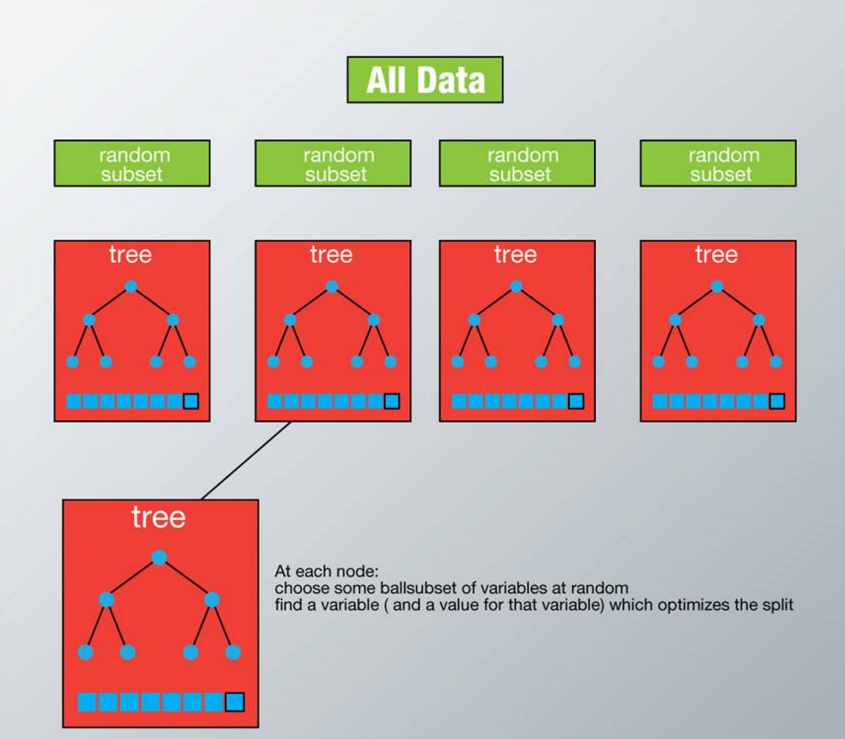
在机器学习中,随机森林是一个包含多个决策树的分类器, 并且其输出的类别是由个别树输出的类别的众数而定。 Leo Breiman和Adele Cutler发展出推论出随机森林的算法。 而 “Random Forests” 是他们的商标。 这个术语是1995年由贝尔实验室的Tin Kam Ho所提出的随机决策森林(random decision forests)而来的。这个方法则是结合 Breimans 的 “Bootstrap aggregating” 想法和 Ho 的”random subspace method”以建造决策树的集合。
基本步骤:
- 假设我们设定训练集中的样本个数为N,然后通过有重置的重复多次抽样来获得这N个样本,这样的抽样结果将作为我们生成决策树的训练集;
- 如果有M个输入变量,每个节点都将随机选择m(m<M)个特定的变量,然后运用这m个变量来确定最佳的分裂点。在决策树的生成过程中,m的值是保持不变的;
- 每棵决策树都最大可能地进行生长而不进行剪枝;
- 通过对所有的决策树进行加总来预测新的数据(在分类时采用多数投票,在回归时采用平均)
Solution
开发流程
收集数据:任何方法
准备数据:转换样本集
分析数据:任何方法
训练算法:通过数据随机化和特征随机化,进行多实例的分类评估
测试算法:计算错误率
使用算法:输入样本数据,然后运行 随机森林 算法判断输入数据分类属于哪个分类,最后对计算出的分类执行后续处理
算法特点
优点:几乎不需要输入准备、可实现隐式特征选择、训练速度非常快、其他模型很难超越、很难建立一个糟糕的随机森林模型、大量优秀、免费以及开源的实现。
缺点:劣势在于模型大小、是个很难去解释的黑盒子。
适用数据范围:数值型和标称型
声纳信号分类
1,收集数据:提供的文本文件
2,准备数据:转换样本集
3,分析数据:手工检查数据
4,训练算法:在数据上,利用 random_forest() 函数进行优化评估,返回模型的综合分类结果
5,测试算法:在采用自定义 n_folds 份随机重抽样 进行测试评估,得出综合的预测评分
6,使用算法:若你感兴趣可以构建完整的应用程序,从案例进行封装,也可以参考我们的代码
- 1, 收集数据:提供的文本文件
样本数据:sonar-all-data.txt
0.02,0.0371,0.0428,0.0207,0.0954,0.0986,0.1539,0.1601,0.3109,0.2111,0.1609,0.1582,0.2238,0.0645,0.066,0.2273,0.31,0.2999,0.5078,0.4797,0.5783,0.5071,0.4328,0.555,0.6711,0.6415,0.7104,0.808,0.6791,0.3857,0.1307,0.2604,0.5121,0.7547,0.8537,0.8507,0.6692,0.6097,0.4943,0.2744,0.051,0.2834,0.2825,0.4256,0.2641,0.1386,0.1051,0.1343,0.0383,0.0324,0.0232,0.0027,0.0065,0.0159,0.0072,0.0167,0.018,0.0084,0.009,0.0032,R
0.0453,0.0523,0.0843,0.0689,0.1183,0.2583,0.2156,0.3481,0.3337,0.2872,0.4918,0.6552,0.6919,0.7797,0.7464,0.9444,1,0.8874,0.8024,0.7818,0.5212,0.4052,0.3957,0.3914,0.325,0.32,0.3271,0.2767,0.4423,0.2028,0.3788,0.2947,0.1984,0.2341,0.1306,0.4182,0.3835,0.1057,0.184,0.197,0.1674,0.0583,0.1401,0.1628,0.0621,0.0203,0.053,0.0742,0.0409,0.0061,0.0125,0.0084,0.0089,0.0048,0.0094,0.0191,0.014,0.0049,0.0052,0.0044,R
0.0262,0.0582,0.1099,0.1083,0.0974,0.228,0.2431,0.3771,0.5598,0.6194,0.6333,0.706,0.5544,0.532,0.6479,0.6931,0.6759,0.7551,0.8929,0.8619,0.7974,0.6737,0.4293,0.3648,0.5331,0.2413,0.507,0.8533,0.6036,0.8514,0.8512,0.5045,0.1862,0.2709,0.4232,0.3043,0.6116,0.6756,0.5375,0.4719,0.4647,0.2587,0.2129,0.2222,0.2111,0.0176,0.1348,0.0744,0.013,0.0106,0.0033,0.0232,0.0166,0.0095,0.018,0.0244,0.0316,0.0164,0.0095,0.0078,R
- 2 准备数据:转换样本集
# 导入csv文件
def loadDataSet(filename):
    dataset = []
    with open(filename, 'r') as fr:
        for line in fr.readlines():
            if not line:
                continue
            lineArr = []
            for featrue in line.split(','):
                # strip()返回移除字符串头尾指定的字符生成的新字符串
                str_f = featrue.strip()
                if str_f.isdigit(): # 判断是否是数字
                    # 将数据集的第column列转换成float形式
                    lineArr.append(float(str_f))
                else:
                    # 添加分类标签
                    lineArr.append(str_f)
            dataset.append(lineArr)
    return dataset
-
3,分析数据:手工检查数据
-
4,训练算法:在数据上,利用 random_forest() 函数进行优化评估,返回模型的综合分类结果
样本数据随机无放回抽样-用于交叉验证
def cross_validation_split(dataset, n_folds):
    """cross_validation_split(将数据集进行抽重抽样 n_folds 份,数据可以重复抽取)

    Args:
        dataset     原始数据集
        n_folds     数据集dataset分成n_flods份
    Returns:
        dataset_split    list集合,存放的是:将数据集进行抽重抽样 n_folds 份,数据可以重复抽取
    """
    dataset_split = list()
    dataset_copy = list(dataset)       # 复制一份 dataset,防止 dataset 的内容改变
    fold_size = len(dataset) / n_folds
    for i in range(n_folds):
        fold = list()                  # 每次循环 fold 清零,防止重复导入 dataset_split
        while len(fold) < fold_size:   # 这里不能用 if,if 只是在第一次判断时起作用,while 执行循环,直到条件不成立
            # 有放回的随机采样,有一些样本被重复采样,从而在训练集中多次出现,有的则从未在训练集中出现,此为自助采样法。从而保证每棵决策树训练集的差异性
            index = randrange(len(dataset_copy))
            # 将对应索引 index 的内容从 dataset_copy 中导出,并将该内容从 dataset_copy 中删除。
            # pop() 函数用于移除列表中的一个元素(默认最后一个元素),并且返回该元素的值。
            fold.append(dataset_copy.pop(index))  # 无放回的方式
            # fold.append(dataset_copy[index])  # 有放回的方式
        dataset_split.append(fold)
    # 由dataset分割出的n_folds个数据构成的列表,为了用于交叉验证
    return dataset_split
- 训练数据集随机化
# Create a random subsample from the dataset with replacement
def subsample(dataset, ratio):   # 创建数据集的随机子样本
    """random_forest(评估算法性能,返回模型得分)

    Args:
        dataset         训练数据集
        ratio           训练数据集的样本比例
    Returns:
        sample          随机抽样的训练样本
    """

    sample = list()
    # 训练样本的按比例抽样。
    # round() 方法返回浮点数x的四舍五入值。
    n_sample = round(len(dataset) * ratio)
    while len(sample) < n_sample:
        # 有放回的随机采样,有一些样本被重复采样,从而在训练集中多次出现,有的则从未在训练集中出现,此为自助采样法。从而保证每棵决策树训练集的差异性
        index = randrange(len(dataset))
        sample.append(dataset[index])
    return sample
- 特征随机化
# 找出分割数据集的最优特征,得到最优的特征 index,特征值 row[index],以及分割完的数据 groups(left, right)
def get_split(dataset, n_features):
    class_values = list(set(row[-1] for row in dataset))  # class_values =[0, 1]
    b_index, b_value, b_score, b_groups = 999, 999, 999, None
    features = list()
    while len(features) < n_features:
        index = randrange(len(dataset[0])-1)  # 往 features 添加 n_features 个特征( n_feature 等于特征数的个数),特征索引从 dataset 中随机取
        if index not in features:
            features.append(index)
    for index in features:                    # 在 n_features 个特征中选出最优的特征索引,并没有遍历所有特征,从而保证了每课决策树的差异性
        for row in dataset:
            groups = test_split(index, row[index], dataset)  # groups=(left, right), row[index] 遍历每一行 index 索引下的特征值作为分类值 value, 找出最优的分类特征和特征值
            gini = gini_index(groups, class_values)
            # 左右两边的数量越一样,说明数据区分度不高,gini系数越大
            if gini < b_score:
                b_index, b_value, b_score, b_groups = index, row[index], gini, groups  # 最后得到最优的分类特征 b_index,分类特征值 b_value,分类结果 b_groups。b_value 为分错的代价成本
    # print b_score
    return {'index': b_index, 'value': b_value, 'groups': b_groups}
- 随机森林
# Random Forest Algorithm
def random_forest(train, test, max_depth, min_size, sample_size, n_trees, n_features):
    """random_forest(评估算法性能,返回模型得分)

    Args:
        train           训练数据集
        test            测试数据集
        max_depth       决策树深度不能太深,不然容易导致过拟合
        min_size        叶子节点的大小
        sample_size     训练数据集的样本比例
        n_trees         决策树的个数
        n_features      选取的特征的个数
    Returns:
        predictions     每一行的预测结果,bagging 预测最后的分类结果
    """

    trees = list()
    # n_trees 表示决策树的数量
    for i in range(n_trees):
        # 随机抽样的训练样本, 随机采样保证了每棵决策树训练集的差异性
        sample = subsample(train, sample_size)
        # 创建一个决策树
        tree = build_tree(sample, max_depth, min_size, n_features)
        trees.append(tree)

    # 每一行的预测结果,bagging 预测最后的分类结果
    predictions = [bagging_predict(trees, row) for row in test]
    return predictions
-
5 测试算法:在采用自定义 n_folds 份随机重抽样 进行测试评估,得出综合的预测评分。
-
计算随机森林的预测结果的正确率
# 评估算法性能,返回模型得分
def evaluate_algorithm(dataset, algorithm, n_folds, *args):
    """evaluate_algorithm(评估算法性能,返回模型得分)

    Args:
        dataset     原始数据集
        algorithm   使用的算法
        n_folds     数据的份数
        *args       其他的参数
    Returns:
        scores      模型得分
    """

    # 将数据集进行随机抽样,分成 n_folds 份,数据无重复的抽取
    folds = cross_validation_split(dataset, n_folds)
    scores = list()
    # 每次循环从 folds 从取出一个 fold 作为测试集,其余作为训练集,遍历整个 folds ,实现交叉验证
    for fold in folds:
        train_set = list(folds)
        train_set.remove(fold)
        # 将多个 fold 列表组合成一个 train_set 列表, 类似 union all
        """
        In [20]: l1=[[1, 2, 'a'], [11, 22, 'b']]
        In [21]: l2=[[3, 4, 'c'], [33, 44, 'd']]
        In [22]: l=[]
        In [23]: l.append(l1)
        In [24]: l.append(l2)
        In [25]: l
        Out[25]: [[[1, 2, 'a'], [11, 22, 'b']], [[3, 4, 'c'], [33, 44, 'd']]]
        In [26]: sum(l, [])
        Out[26]: [[1, 2, 'a'], [11, 22, 'b'], [3, 4, 'c'], [33, 44, 'd']]
        """
        train_set = sum(train_set, [])
        test_set = list()
        # fold 表示从原始数据集 dataset 提取出来的测试集
        for row in fold:
            row_copy = list(row)
            row_copy[-1] = None
            test_set.append(row_copy)
        predicted = algorithm(train_set, test_set, *args)
        actual = [row[-1] for row in fold]

        # 计算随机森林的预测结果的正确率
        accuracy = accuracy_metric(actual, predicted)
        scores.append(accuracy)
    return scores
- 6 ** 使用算法**:若你感兴趣可以构建完整的应用程序,从案例进行封装,也可以参考我们的代码
预测收入情况
如何利用某一个人的年龄(Age)、性别(Gender)、教育情况(Highest Educational Qualification)、工作领域(Industry)以及住宅地(Residence)共5个字段来预测他的收入层次。 预测的目标收入层次 :
- Band 1 : Below $40,000
- Band 2: $40,000 – 150,000
- Band 3: More than $150,000
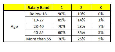
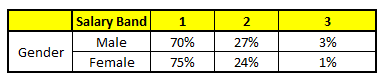
算法过程 随机森林中每一棵树都可以看做是一棵CART(分类回归树),这里假设森林中有5棵CART树,总特征个数N=5,我们取m=1(这里假设每个CART树对应一个不同的特征)。
| CART 1 : Variable Age | CART 2 : Variable Gender |
|---|---|
 |
 |
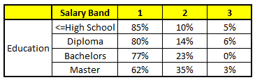
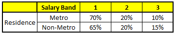
| CART 3 : Variable Education | CART 4 : Variable Residence |
|---|---|
 |
 |
| CART 5 : Variable Industry | - |
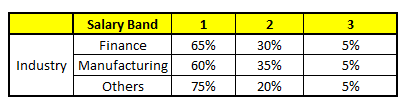 |
我们要预测的某个人的信息如下:
- Age : 35 years ; 2. Gender : Male ; 3. Highest Educational Qualification : Diploma holder; 4. Industry : Manufacturing; 5. Residence : Metro.
根据这五棵CART树的分类结果,我们可以针对这个人的信息建立收入层次的分布情况:
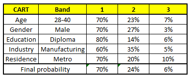 最后,我们得出结论,这个人的收入层次70%是一等,大约24%为二等,6%为三等,所以最终认定该人属于一等收入层次(小于$40,000)。
Programing Sample
Sklearn
#Import Library
from sklearn.ensemble import RandomForestClassifier

#Assumed you have, X (predictor) and Y (target) for training data set and x_test(predictor) of test_dataset
# Create Random Forest object
model= RandomForestClassifier()

# Train the model using the training sets and check score
model.fit(X, y)

#Predict Output
predicted= model.predict(x_test)
# sklearn_rf.py
import pandas as pd
from sklearn.ensemble import RandomForestClassifier

df = pd.read_csv('sklearn_data.csv')
train, test = df.query("is_date != -1"), df.query("is_date == -1")
y_train, X_train = train['is_date'], train.drop(['is_date'], axis=1)
X_test = test.drop(['is_date'], axis=1)

model = RandomForestClassifier(n_estimators=50,
                               criterion='gini',
                               max_features="sqrt",
                               min_samples_leaf=1,
                               n_jobs=4,
                           )
model.fit(X_train, y_train)
print model.predict(X_test)
print zip(X_train.columns, model.feature_importances_)

调用RandomForestClassifier时的参数说明:
n_estimators:指定森林中树的颗数,越多越好,只是不要超过内存;
criterion:指定在分裂使用的决策算法;
max_features:指定了在分裂时,随机选取的特征数目,sqrt即为全部特征的平均根;
min_samples_leaf:指定每颗决策树完全生成,即叶子只包含单一的样本;
n_jobs:指定并行使用的进程数;
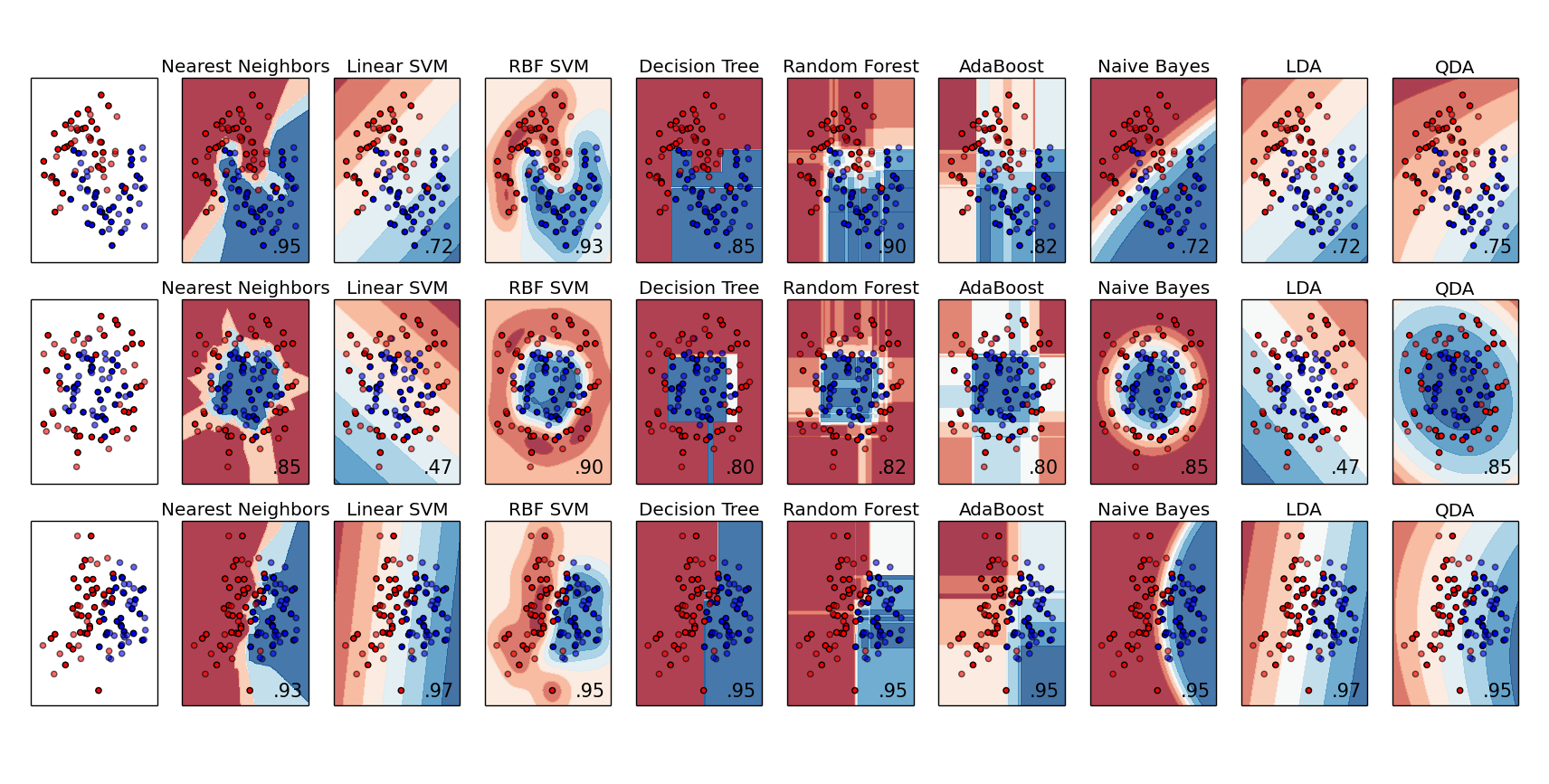
Sklearn 与其他算法比较
import numpy as np
import matplotlib.pyplot as plt
from matplotlib.colors import ListedColormap
from sklearn.cross_validation import train_test_split
from sklearn.preprocessing import StandardScaler
from sklearn.datasets import make_moons, make_circles, make_classification
from sklearn.neighbors import KNeighborsClassifier
from sklearn.svm import SVC
from sklearn.tree import DecisionTreeClassifier
from sklearn.ensemble import RandomForestClassifier, AdaBoostClassifier
from sklearn.naive_bayes import GaussianNB
from sklearn.lda import LDA
from sklearn.qda import QDA

h = .02  # step size in the mesh

names = ["Nearest Neighbors", "Linear SVM", "RBF SVM", "Decision Tree",
         "Random Forest", "AdaBoost", "Naive Bayes", "LDA", "QDA"]
classifiers = [
    KNeighborsClassifier(3),
    SVC(kernel="linear", C=0.025),
    SVC(gamma=2, C=1),
    DecisionTreeClassifier(max_depth=5),
    RandomForestClassifier(max_depth=5, n_estimators=10, max_features=1),
    AdaBoostClassifier(),
    GaussianNB(),
    LDA(),
    QDA()]

X, y = make_classification(n_features=2, n_redundant=0, n_informative=2,
                           random_state=1, n_clusters_per_class=1)
rng = np.random.RandomState(2)
X += 2 * rng.uniform(size=X.shape)
linearly_separable = (X, y)

datasets = [make_moons(noise=0.3, random_state=0),
            make_circles(noise=0.2, factor=0.5, random_state=1),
            linearly_separable
            ]

figure = plt.figure(figsize=(27, 9))
i = 1
# iterate over datasets
for ds in datasets:
    # preprocess dataset, split into training and test part
    X, y = ds
    X = StandardScaler().fit_transform(X)
    X_train, X_test, y_train, y_test = train_test_split(X, y, test_size=.4)

    x_min, x_max = X[:, 0].min() - .5, X[:, 0].max() + .5
    y_min, y_max = X[:, 1].min() - .5, X[:, 1].max() + .5
    xx, yy = np.meshgrid(np.arange(x_min, x_max, h),
                         np.arange(y_min, y_max, h))

    # just plot the dataset first
    cm = plt.cm.RdBu
    cm_bright = ListedColormap(['#FF0000', '#0000FF'])
    ax = plt.subplot(len(datasets), len(classifiers) + 1, i)
    # Plot the training points
    ax.scatter(X_train[:, 0], X_train[:, 1], c=y_train, cmap=cm_bright)
    # and testing points
    ax.scatter(X_test[:, 0], X_test[:, 1], c=y_test, cmap=cm_bright, alpha=0.6)
    ax.set_xlim(xx.min(), xx.max())
    ax.set_ylim(yy.min(), yy.max())
    ax.set_xticks(())
    ax.set_yticks(())
    i += 1

    # iterate over classifiers
    for name, clf in zip(names, classifiers):
        ax = plt.subplot(len(datasets), len(classifiers) + 1, i)
        clf.fit(X_train, y_train)
        score = clf.score(X_test, y_test)

        # Plot the decision boundary. For that, we will assign a color to each
        # point in the mesh [x_min, m_max]x[y_min, y_max].
        if hasattr(clf, "decision_function"):
            Z = clf.decision_function(np.c_[xx.ravel(), yy.ravel()])
        else:
            Z = clf.predict_proba(np.c_[xx.ravel(), yy.ravel()])[:, 1]

        # Put the result into a color plot
        Z = Z.reshape(xx.shape)
        ax.contourf(xx, yy, Z, cmap=cm, alpha=.8)

        # Plot also the training points
        ax.scatter(X_train[:, 0], X_train[:, 1], c=y_train, cmap=cm_bright)
        # and testing points
        ax.scatter(X_test[:, 0], X_test[:, 1], c=y_test, cmap=cm_bright,
                   alpha=0.6)

        ax.set_xlim(xx.min(), xx.max())
        ax.set_ylim(yy.min(), yy.max())
        ax.set_xticks(())
        ax.set_yticks(())
        ax.set_title(name)
        ax.text(xx.max() - .3, yy.min() + .3, ('%.2f' % score).lstrip('0'),
                size=15, horizontalalignment='right')
        i += 1

figure.subplots_adjust(left=.02, right=.98)
plt.show()
Spark
from pprint import pprint
from pyspark import SparkContext
from pyspark.mllib.tree import RandomForest
from pyspark.mllib.regression import LabeledPoint

sc = SparkContext()
data = sc.textFile('spark_data.csv').map(lambda x: x.split(',')).map(lambda x: (float(x[0]), int(x[1]), int(x[2]), float(x[3]), int(x[4]), int(x[5])))
train = data.filter(lambda x: x[5]!=-1).map(lambda v: LabeledPoint(v[-1], v[:-1]))
test = data.filter(lambda x: x[5]==-1)#.map(lambda v: LabeledPoint(v[-1], v[:-1]))

model = RandomForest.trainClassifier(train,
                                     numClasses=2,
                                     numTrees=50,
                                     categoricalFeaturesInfo={1:2, 2:2, 4:3},
                                     impurity='gini',
                                     maxDepth=5,
                                 )

print 'The predict is:', model.predict(test).collect()
print 'The Decision tree is:', model.toDebugString()